Northcentral Technical College (NTC) in Wisconsin has experienced a crippling cyber attack that shut down most of its classes from Monday through Wednesday. The cyber attack triggered system outages all over the school causing school officials to issue a public notice on the homepage of the college website that read:
“We apologize for the inconvenience but we are continuing to experience IT system outages. NTC’s Information Technology team is working diligently to bring information systems back online. We will continue to post updates to this page as they are available.”
Cyber forensics investigation underway
The college would not release any specific information about the data that was lost, but they did reassure their students and faculty that no one’s personal data was stolen. They have since hired a cyber forensics team who will perform a thorough investigation of the cyber intrusion. School officials want to know what type of information was targeted and whether any data was lost or compromised.
Marketing and public relations director, Kelsi Seubert, commented saying, “NTC’s Information Technology team is working extremely hard to bring information systems back online and we will communicate additional updates to students and staff as they are available.”
Seubert also sent an email out to students and faculty that reassured everyone that an investigation was underway but would require some time to complete. She also mentioned that the initial attempted hack occurred on June 4th.
The school has stated that all classes will be resumed on Thursday and that campus life would soon return to normal. A few classes that were not impacted by the breach were carried out as usual.
Summer school
The summer class schedule had just begun on Monday with students showing up to take advantage of Northcentral’s summer learning programs. The school offers a unique array of subjects ranging from technical diplomas to Information Technology training. Students can take summer courses to get additional credits so they can graduate sooner, or they can catch up on classes they may have missed.
The school has a flexible curriculum that includes virtual educational opportunities, online classes, late-start classes, winter enrollments, and many others. They offer associate’s degrees, certifications, and technical diplomas. In the accelerated credits program, students can get three credits in three weeks by taking augmented versions of the class.
Cyber breaches on the rise
Security breaches and cyber-attacks have become common in the news. Though it seems like everyone should know by now what it takes to prevent them, cyber thieves are escalating their tactics with each new attack.
In over 90 percent of these events, human error is to blame. A school official or teacher may have inadvertently clicked on a suspicious link. The latest phishing attacks include emails that look almost identical to what you might get from a bank or credit card company. Often, the email will say that something is wrong with your account. Cybercriminals use fear to gain access to your personal log-in information. An email might say something like:
“Alert! You have been locked out of your ABC Credit Card account due to suspicious activity. Click the link below to sign in and change your password.”
Once you click that link, you may be redirected to a phony website where the hackers will steal your password and username. Now they have legitimate access to your credit card account. They can go online and buy the merchandise having it shipped to an address overseas.
In this situation, never click on the link that’s embedded in the email. Instead, open a fresh page in your browser and navigate to your credit card account the way you normally would. Log in and check your messages. In most cases, there’s absolutely nothing wrong with the account; it was just a ruse to get you, the consumer, to give away your password and username to cyber thieves on the other side of the world.
Third party vendors
Colleges and schools do business with a wide number of third-party vendors. If these vendors have access to any of your important data, then they should be thoroughly vetted in advance. Though a school or business cannot control the activities of third-party vendors, it’s important to make every effort to ensure that they are observing stringent security regulations.
Faculty training
All school faculty should attend regular security meetings to learn about the latest cyber threats and how to avoid them. Training employees and teachers have proven to reduce the number of cyber breaches. Training should include facts about how security breaches occur and what to do to stop them. Faculty should understand the difference between ransomware and malware. They should be familiar with the many types of phishing and spear phishing attacks. These are just a few of the many ways an organization can protect itself against cyber- attacks.
Northcentral Technical College life returning to normal
Though school administrators have reassured everyone that no financial, personal, or confidential information was stolen, the investigation into what happened is only just beginning. It often takes months for an organization to realize the full extent of a cyber-breach. It can be years before the true cost of the security breach is fully understood.
Northcentral Technical College located in Wausau, Wisconsin, is a community college and member of 16 schools in the Wisconsin Technical College System.
Phishing is one of the most dangerous forms of identity theft. It’s usually presented in the form of pop-ups or spam emails. The majority of account takeovers come from simple phishing attacks where someone in an organization gets tricked into releasing private credentials and information.
Never give your contact details over the phone. This includes user IDs, passwords, Social Security numbers or other personal information. The IRS, a bank, Microsoft or other legitimate organizations will never call and ask you for this information.
Be suspicious of every email. Never click on a link or open an attachment in an email without verifying the sender’s identity and intent. Always be suspicious of any email asking you to verify information, send money or pay an overdue invoice.
Don’t respond to a CEO request for urgent payments. There have been numerous cases where a CEO’s contact information was spoofed and used to convince employees to send money to scammers. Contact the CEO directly to determine if this is a fraudulent request.
It doesn’t take long for a hacker to steal your company secrets.
More Tips To Share With Your Staff
Be cautious about opening attachments. They may contain malware that can infect your computer.
Type in URLs and email addresses, don’t click the link email.
Use Two-Factor Authentication. It requires both your password and an additional piece of information to log in to your account.
Always update your applications and operating system. Don’t delay, as they will protect your computer and network from the latest threats.
Back up your files to an external hard drive or cloud storage to ensure you have a duplicate of all your files and applications if your network is compromised.
What Else You Can Do
Ask our IT Security Experts to provide a layered and managed security protection for your technology. A layered security approach combines best-in-class firewalls, web-filtering, and software-update services to protect your network from viruses, malware, and hackers.
Tell your employees to let you know if they experience the following:
They can’t open their files, or they get error messages saying a file is corrupted or contains the wrong extension.
A window pops up with a ransomware program they can’t close. This window may contain a message about paying a ransom to unlock files.
A message says that a countdown has started for a ransom to decrypt files and that it will increase over time.
They see files in their directories with names like “How to decrypt files.txt or decrypt_instructions.html.”
Have questions?
Our team can conduct Security Awareness Training for your employees. This way they’ll know what to do if they get a phishing email.
This great tip comes from Karen Turner of Turner Efficiency in Calgary, Alberta, Canada.
Draw a line down your page so you can immediately distinguish notes from tasks/to-do’s/follow-up actions.
When has a meeting or a class ended without you having to do some follow-up? Not often, I bet. That’s why a line is so effective.
Use the outside 1/3 of the page for all the “after” actions so they’re easy to see, especially when you fan your notebook’s edge.
Use the inside 2/3 of the page for notes.
Finally, for fast filing, rip out the page and put the 2/3 notes part in the file and the 1/3 actions part on your desk for follow-up.
Granted, this won’t win you any tidiness awards, but it will ensure that your files are compliant and, at the very least, save you from searching through notebooks.
The new features in Outlook are designed to help users save time and be more productive. Since we spend so much time writing and answering emails, this is one area where most of us would love to be able to get done faster. Microsoft designed Outlook with lots of thought and effort. In addition, they add exciting features every year or so. They do plenty of solid research when designing all their products because they believe in finding out what users are asking for and providing that.
Intuitive design
You can see the planning that went into developing this version of Outlook. Most people will pick up how the new features are used pretty quickly though since this version is similar-looking to older ones. All Office 365 products share a similar look and feel in their design. The Ribbon contains many of the same features whether you’re using Word, Powerpoint, or Outlook.
Outlook’s new design is so streamlined that the new features transform the way you connect to your people and technology. It will infuse power into every productivity task. It comes with better security to ward off hackers. Keeping your email safe and secure is an important job. Today’s software programs and apps must contain higher level security features in order to address the growing number of data breaches going on all over the world. Microsoft does a good job of incorporating better security measures than many other companies.
There are a lot more new things to see and do in the new Outlook 2018. It can be configured to give users the convenience they’re looking for in an email program. Once you learn the ins and outs of the program, you can fly through otherwise boring tasks.
Below, we check out 5 of the coolest new features in Outlook. They should help you get your work done each day with time to spare.
Multiple time zones
Traveling around the world? Trying to sync appointments with people on various continents? Whether you’re just flying to Chicago or going to Tanzania, you can configure Outlook to set up meetings based on whatever time zone you choose. Appointment times will sync up depending on where everyone is. Each person is given the meeting time in their own time zone so no one will be late for the meeting. This is a super convenient feature that everyone will appreciate since the business world is now a global affair.
It’s easy to set this feature up. Open the Windows version of Outlook, then add an event by selecting File > Options > Calendar Time Zones. Now choose the option, “Show a second-time-zone.” If you’re using Outlook on the web, you should click on the drop-down arrow called “Time Zone.” This item can be found in your Calendar. If using a Mac, you can add extra time zones by navigating to Outlook > Preferences > Calendar Time Zones. With a little practice, you can become a pro at setting up various meetings with customers and team members around the world.
RSVP
Invite the whole crew to a picnic at the lake. After all, fun outdoor events are a good way to build camaraderie. Outlook makes it easy to send invitations, whether it’s a party, picnic, big meeting with the boss or just a lunch date. RSVP keeps track of who is coming (Tracking Option) and whether RSVP’s have been replied to. You’ll get reminders about the event based on how you set it up. You can get daily or weekly reminders. This feature is offered for both the meeting organizer and attendees.
Office Lens for Android
This is a really simple but helpful feature that lets you integrate the Microsoft Office Lens into your Outlook email program. It only works for Android though. It’s easy to use but very useful. Simply open an email that you want to send to someone. Next, tap the photo icon while creating your message. Now you can take a pic of anything and embed it in the document. You might want to include a photo of a colleague sitting across from you. You could snap a photo of a whiteboard or even a document. Outlook optimizes the photo, then embeds it into your email. There are countless uses for this handy feature.
BCC warning
We’ve all accidentally sent emails to the wrong person. Sometimes, it can be quite embarrassing. This is often the case if you get “BCC’d” on an email and decide to reply. Often people use BCC because they do not want the other people included in the email to know that a specific person got a copy of it. In the new Outlook, if you should hit “Reply All” to an email where you were BCC’d, you will get a warning message. It may say something like, “You were bcc’d on this email. Are you sure you want to reply to all?” We all need someone around to double check our actions from time to time and this feature might save you some embarrassment one day.
Bill-pay reminders
What if an email program could remind you when bills are due? Wouldn’t that be convenient? Outlook has the ability to identify the bills in your inbox, then put together a summary of them each day. This will appear at the top of your email when you first turn it on. Two days before the due date for each bill, you’ll get a reminder. The email program automatically adds an event to your calendar for the actual day the bill is due. Now there’s no excuse for forgetting to pay the light bill.
Conclusion
Outlook has many more really helpful features designed to make your life a little easier. Once you learn all the tips and tricks, you’ll cut time off your work day and get things done more efficiently. If you’d like to learn more about the new Outlook 2018 features, please visit this article.
According to a recent survey, around 29 percent of companies named security as the major problems in the upcoming years. The current percentage is a ten percent increase from last year’s survey results. While security is the biggest problem, efficiency and workflow was a close second, at 26 percent. Apart from cybersecurity and problems pertaining to privacy, emerging technology and infrastructure management have also been ranked as the top technological challenges faced by companies; regarding of the industry they belong to.
Challenges faced by tech companies
While firms do face these major challenges, coming up with a solution for them is a problem because half of the companies that cited security as a big problem don’t have the money needed to deal with the problem. Half of the respondents claimed that their firm’s budget was the same as last year while 8% of them stated that the budget allocated to the IT department was smaller this year. Another research also suggests that a large part of global companies, up to 55%, only have an IT audit assessment on a less-frequent basis; most commonly once a year.
It is a difficult task for security professionals to get the budget they require for setting up a proper, well-developed cybersecurity program. The problem is that security professionals are only handed the budget after there has been a major data breach or if there has been an incident that has left a negative impact on the company. A number of organizations find it hard to quantify security or put a monetary value on it.
With news filled about phishing scams and hacking incidents and social media websites talking about privacy, one can easily understand why security is such a concern. For instance, just last year in May, companies in more than 150 countries had been targeted. The targeted companies included big names such as NHS, FedEx, and Honda.
Just like law firms, tech firms also store tremendous amounts of sensitive data about users, which is why it is crucial for them to employ high-security levels. A lack of security on the part of tech firms not only shows negligence but also puts all the users at risk who’s data is stored with the company.
What security challenges do tech firms face?
The challenges to cybersecurity are regularly developing and are becoming more severe; making it vital for tech firms to stay on top of their game and constantly work on finding solutions, so they stay safe from security attacks. Mentioned below are a few of the common kinds of threat that tech companies can face:
Malware
Malware is highly common. Not only is it present abundantly on the internet, but it is also the tool that a majority of cybercriminals use for obtaining their goal. Whether it is for locking up computers and charging them for obtaining their goal or it is for infiltrating an organization and stealing confidential information; malware is the best tool. Similarly, malware can also be used for making public statements and getting people’s attention. In each cybersecurity incident, malware always has a role. In fact, it can also be used as a pivot into the company.
Users
While this might seem surprising but users are a threat too. For instance, the threat can come from the inside, i.e., a malicious employee, or it could also be because of accidental user actions.
Spear phishing
Another tool that is becoming more common these days is spear phishing, primarily because it is quite effective. Hardly anyone thinks twice before opening any PDF document or a Word document. Many of us, in fact, use it regularly for work without thinking. This routine of not giving a second thought before opening a document is exactly the factor that criminals count on.
For all these security threats, the solution is simple; user education. For any organization, it is crucial to teach employees to first think before clicking on anything; whether it is a link or a document. While user education is important, it doesn’t mean that technology selection should be neglected. Enterprise systems can provide a sufficient amount of security if their users are given the right cybersecurity training and know how to use the systems correctly. While this requires more money and more time, the training is crucial for keeping the firm’s data protected.
Furthermore, another step that firms can take is to use email gateway technologies that can help get rid of the malicious emails before it goes into the user’s inbox. This simple measure can go a long way when it comes to protecting the firm from spear phishing.
Bottom line
It cannot be denied that the industry is filled with challenges, that increase in difficulty with each passing year. However, the good news is that all problems can be solved if only firms make use of passion, ingenuity, and a systematic thought process for solving them.
This is the final of a three-part series about using Microsoft Excel 2016. It will cover some of the more advanced topics. If you aren’t great with numbers, don’t worry. Excel does the work for you. With the 2016 version of Excel, Microsoft really upped its game. Excel’s easy one-click access can be customized to provide the functionality you need.
If you haven’t read Part I and Part II of this series, it’s suggested that you do so. The webinar versions can also be found on our site or on YouTube.
This session will discuss the following:
More with Functions and Formulas
Naming Cells and Cell Ranges
Statistical Functions
Lookup and Reference Functions
Text Functions
Documenting and Auditing
Commenting
Auditing Features
Protection
Using Templates
Built-In Templates
Creating and Managing Templates
More With Functions And Formulas
Naming Cells And Cell Ranges
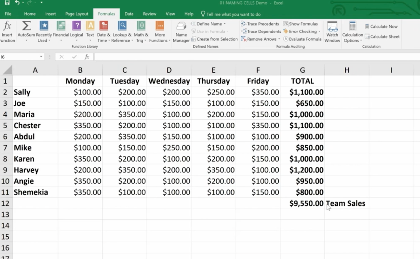
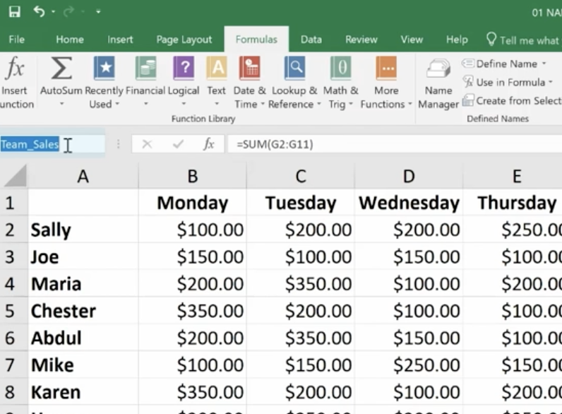
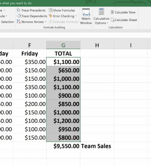
How do you name a cell? You do so by the cell’s coordinates, such as A2 or B3, etc. When you write formulas using Excel’s coordinates and ranges you are “speaking” Excel’s language. However, this can be cumbersome. For example, here G12 is significant because it refers to our Team Sales.
You can teach Excel to speak your language by naming the G12 cell Team Sales. This will have more meaning to you and your teammates. The benefits of naming cells in this fashion are that they are easier to remember, reduce the likelihood of errors, and use absolute references (by default).
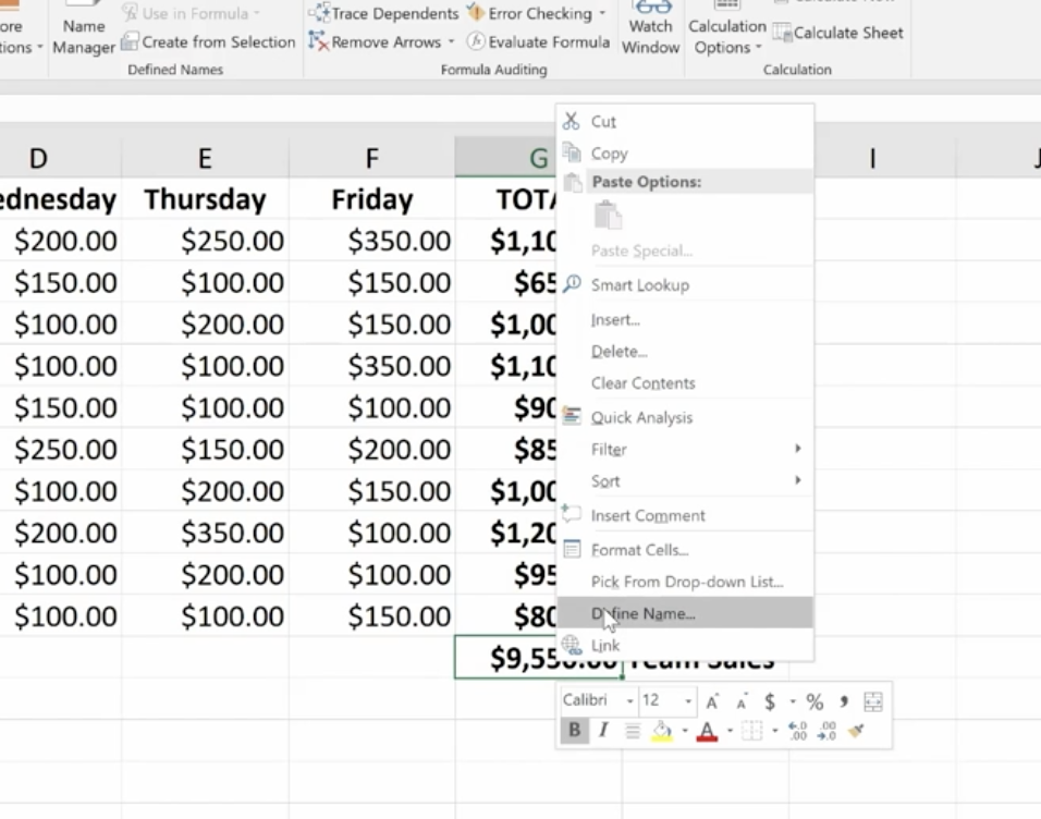
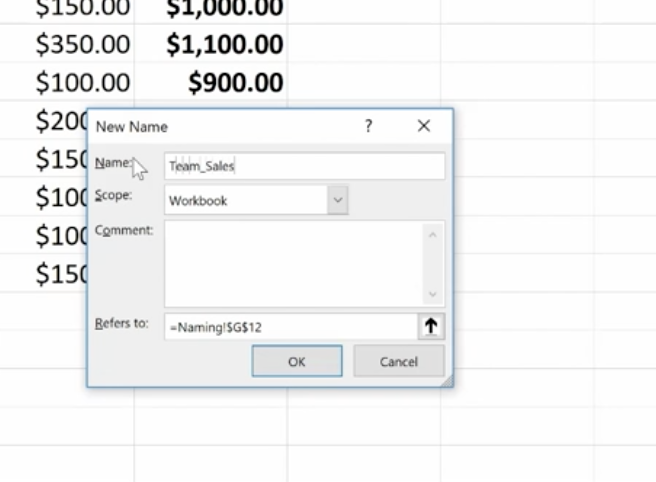
To name our G12 cell Team Sales, right-click on the cell, choose Define Name, and type “Team Sales” into the dialog box. You can also add any comments you want here. Then click Ok.
Another way to do this is to click on the G12 cell and go up to the Name Box next to the Formula Bar, then type your name there.
And, there’s a third option at the top of the page called “Define Cells” that you can use.
Notice that there’s an underscore between Team and Sales (Team_Sales). There are some rules around naming cells:
You’re capped at 255 characters.
The names must start with a letter, underscore or a backslash (\).
You can only use letters, numbers, underscores or periods.
Strings that are the same as a cell reference, for example B1, or have any of the following single letters (C,c,R,r) cannot be used as names.
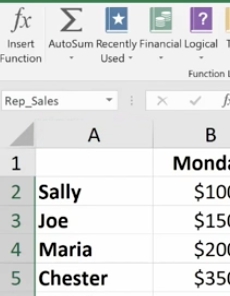
How To Name A Range
Highlight an entire range of cells and name your range (we’re doing this in the upper left-hand corner).
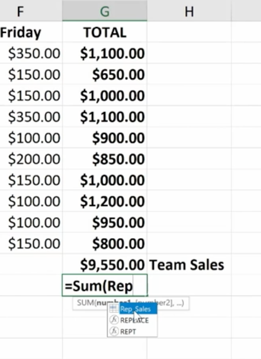
Then you can easily use the name to produce the sum you need:
You won’t have to go back and forth from spreadsheet to spreadsheet clicking on specific cells to calculate your formula. You simply key in the name of the cell range you want to add. Just be sure to remember the names as you build your spreadsheets over time.
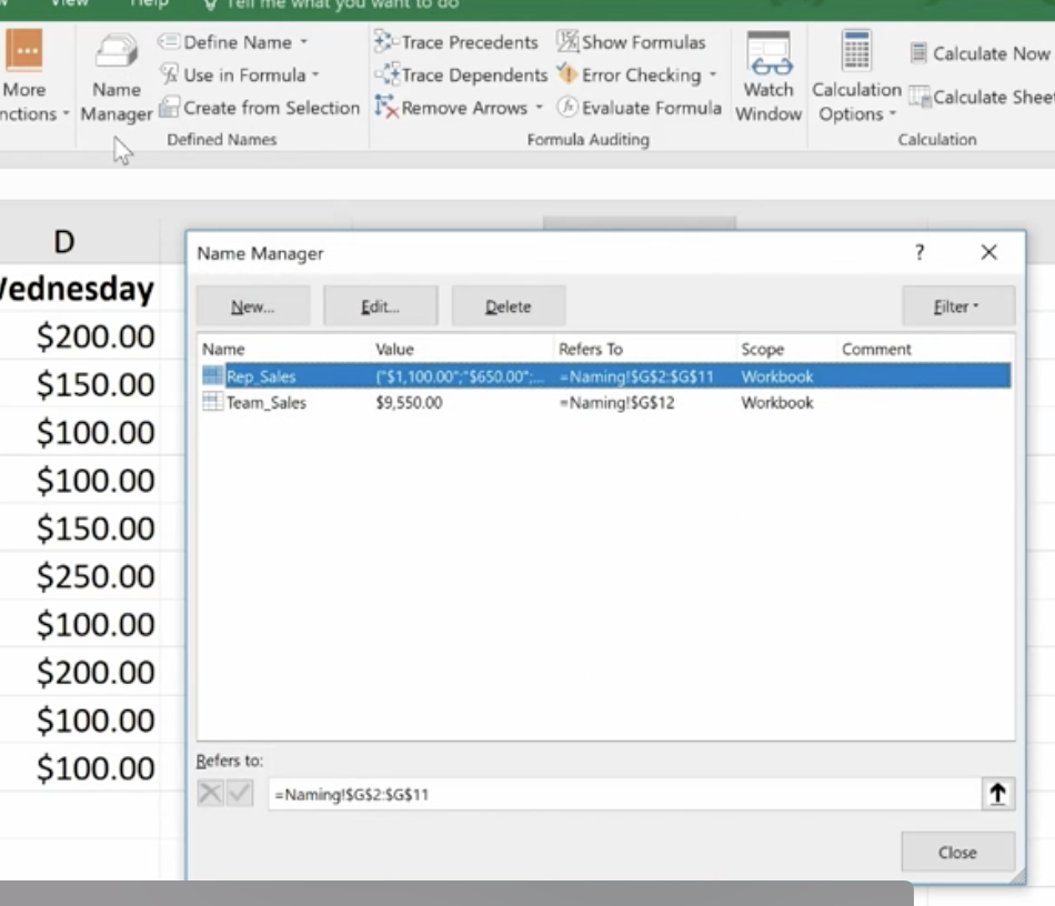
If you ever make a mistake or want to change names, you can go to Name Manager to do this.
Remember that if you move the cells, the name goes with it.
Statistical Functions
The three statistical functions are:
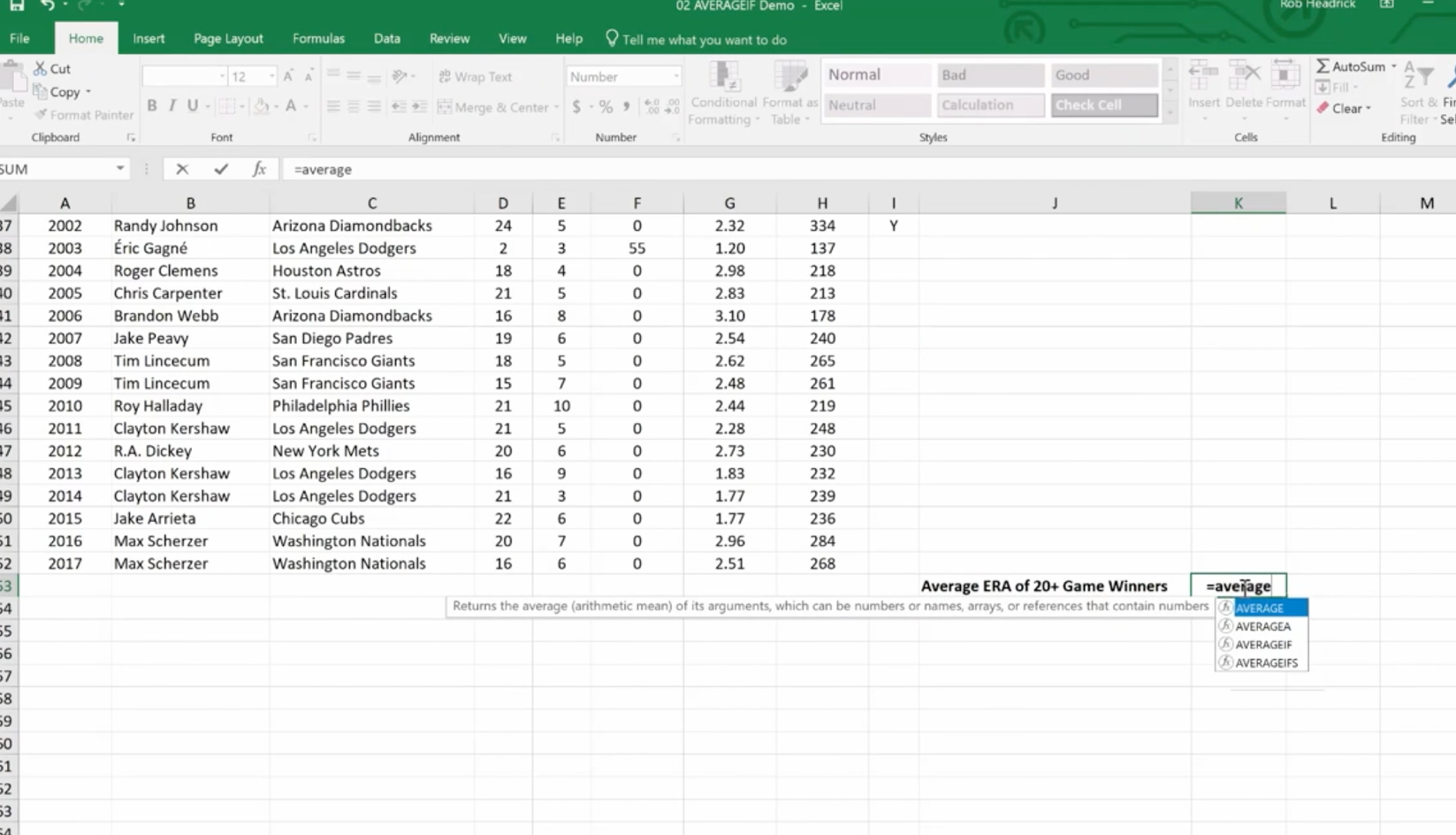
Average If
Count If
Sum If
The Average If can be used to figure out the average of a range based on certain criteria. Here we’re going calculate the Average If of the ERA of 20+ Game Winners from the spreadsheet we developed in our last session.
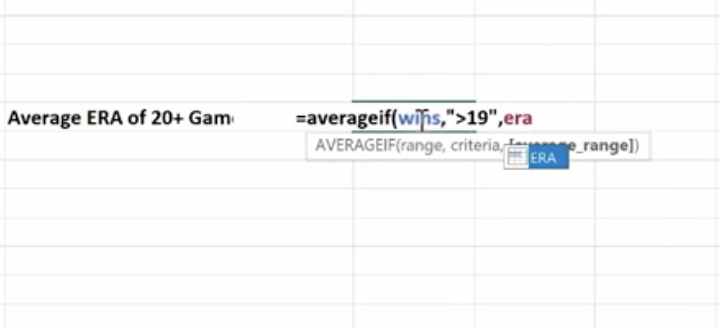
We’ve already named some of our cell ranges (wins, era). And we want to know the average greater than 19.
Hit Enter and you have the average.
You can use this feature across a wide variety of scenarios. For example, if you wanted to know the average sales of orders above a certain quantity – or units sold by a particular region, or the average profit by a distinct quarter.
Count If is used for finding answers to questions like, “How many orders did client x place?” “How many sales reps had sales of $1,000 or more this week?” or “How many times have the pitchers of the Philadelphia Phillies won the Cy Young Award?”
As you can imagine, it’s essential that you type in the text exactly the way you named that particular cell.
Hit Enter and you get your answer
Now we’re going to use the Sum If function to calculate the number of strikeouts by the pitchers on this list who are in the Baseball Hall of Fame.
Sum If is a good way to perform a number of real-world statistical analyses. For example, total commissions on sales above a certain price, or total bonuses due to reps who met a target goal, or total earnings in a particular quarter year-over-year.
Lookup and Reference Functions
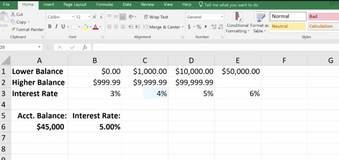
These are designed to ease the finding and referencing of data, especially in large tables. Here, cells A1 and E3 relate to a variable interest rate that is paid on a bank account. For balances under $1,000, the interest rate is 3% – between $1,000 and $10,000, the interest rate is 4%, etc.
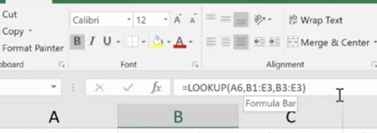
Cell A6 shows the balance of a specific account. The Lookup Function is used in B6. It looks up the interest rate and applies it to the account balance of $45,000. This is what the formula looks like in the bar at the top:
The vector form of the Excel Lookup Function can be used with any two arrays of data that have one-to-one matching values. For example, two columns of data, two rows of data, or even a column and a row would work, as long as the Lookup Vector is ordered (alphabetically or numerically), and the two data sets are the same length.
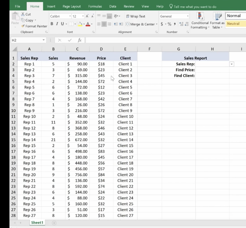
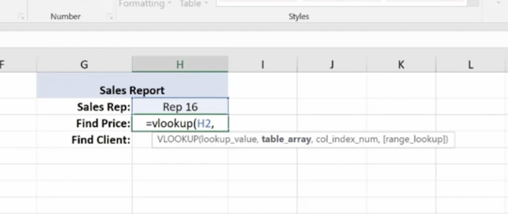
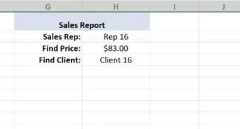
V Lookup and H Lookup are used to pull information into reports. We’re going to use Report Setup. Here, we have a worksheet that references salespeople, sales data, pricing, revenue, and the clients that they sold to. You’ll see on the top right where we set up a report with names referencing sales data.
You can access the sales reps in the drop-down menu. Pick a rep and use the V Lookup Function to find the price.
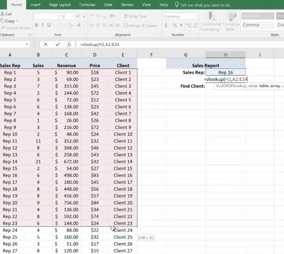
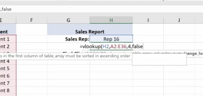
To Find Price, key in =vlookup and the corresponding cell number for Rep 16, plus the table array which is the entire table not including the header at the top.
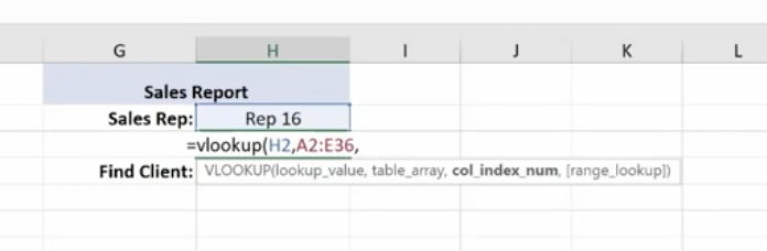
Then you need the column index number. This is the number of columns to the right of your lookup value column, which is column A. It’s the 4th column from column A (Price).
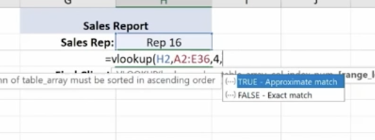
Enter 4,
For range lookup we’re using true or false. We are entering false here.
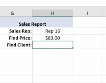
Hit Enter and this is what you have for your Find Price value.
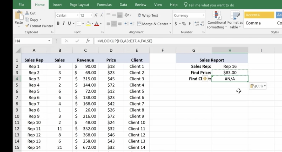
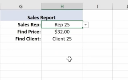
Now we’ll do a similar V Lookup for the Client. Copy and Paste:
Make the necessary changes in your formula:
Client 16 goes with Rep 16.
Note: If you change the Sales Rep, all the corresponding values will change.
If you have a lot of data and long tables, V Lookup helps you find information easily. The V stands for Vertical (or by column), because columns are vertical. H Lookup is for Horizontal-like column headers.
Text Functions
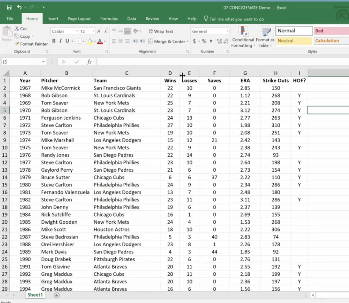
Text Functions contain some very powerful tools to adjust, rearrange and even combine data. These functions are used for worksheets that contain information and function as a database such as mailing lists, product catalogs, or even Cy Young Award Winners.
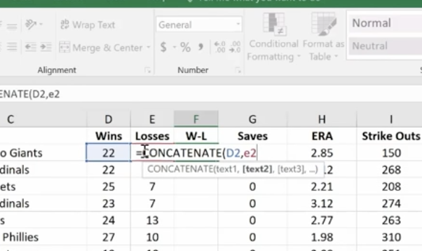
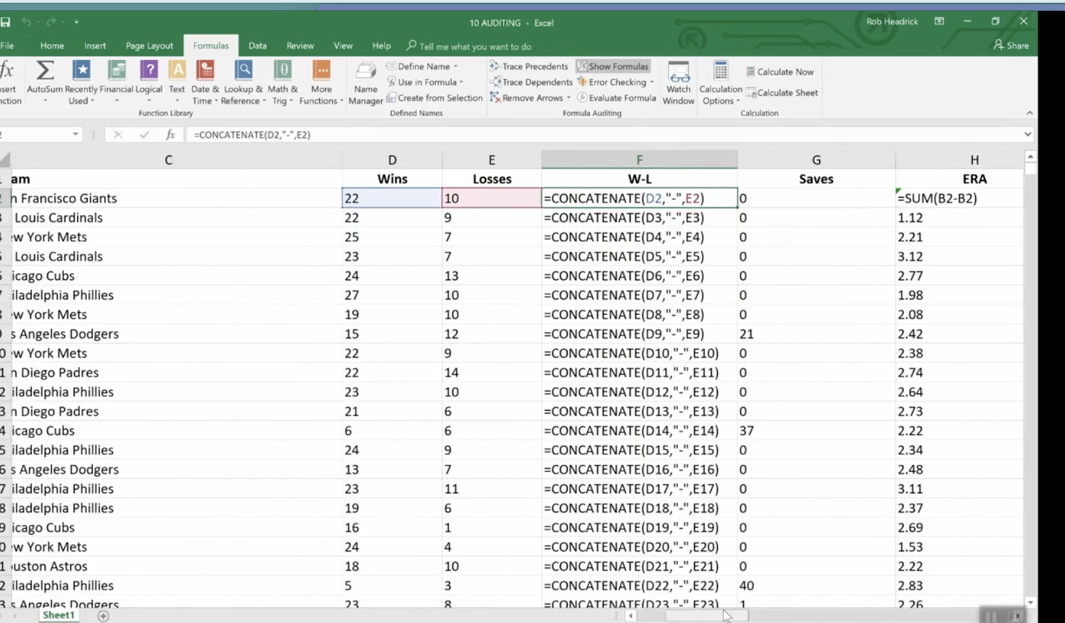
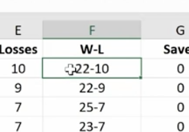
The first text function we’ll show you is concatenate. It links things together in a chain or series. Here, we have our Cy Young list. But we no longer need to see our Wins and Losses in a separate column.
To do this easily rather than manually, create a new column where your data will reside.
Hit Enter
Now, just go in and hide the Wins and Losses columns. Don’t delete them or your new column will have a reference error.
If you do want to delete the Wins and Losses columns, you must first make a new column. Copy the W-L numbers and Paste Value in the new column. This way you’ve moved from a formula to the new information. If you delete your source information without taking this step you’ll be left with nothing.
Combine as many columns as you need with the concatenate function to make the data appear as you need it to.
The Left Mid and Right Functions
These are used to tell Excel that you only want part of a text string in a particular cell. Here, we have a product list and product IDs that tell us the date of manufacturer, the item number, and the factory where it was made. We’re going to pull the data out so we can put it in columns to use in different ways.
We use the Mid Function here.
This works because each of the product IDs are the same length. If they were different lengths you’d have to do something more creative.
Documenting and Auditing
You want to make your Excel files easy to understand for both yourself and others who need to use them – and this includes auditors. An organized worksheet results in clear error-free data and functions.
Commenting
The purpose of commenting is to provide notes to yourself or especially to others. Comments can include reminders, explanations or suggestions.
You’ll find the New Comment button at the top under the Review Menu. Simply click the cell where you want the comment to go and click New Comment. Then type your comment and click outside the box to close it. The comment will disappear but it’s still there. Anywhere you see a red flag, there’s a comment.
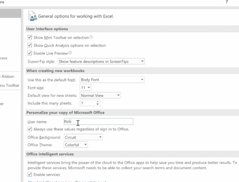
If your name doesn’t appear in the comment, go to File>Options>General and personalize your copy of Excel (in this case Microsoft Office) under the User Name. You won’t need to go back and change each comment; Excel will do this for you.
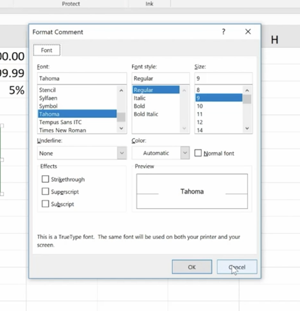
To format a comment, click inside the comment box and a drop down will come up where you can format the text.
You can change the color of the box and lines around the box. Some managers have different colors for members of their teams.
If you change the default color, it will change that for all your Microsoft products.
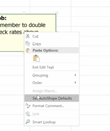
To delete a comment, go to the cell that hosts it, then go up and hit delete.
If you have a lot of comments, grab the handle on the box and resize it.
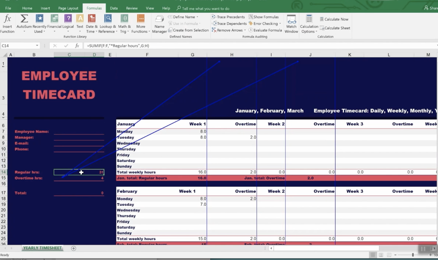
Auditing
What we really mean is formula auditing. This is an advanced way to check your work.
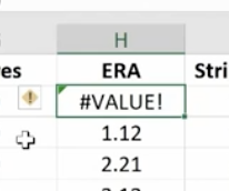
The yellow diamond on the left of this cell indicates that there’s an error.
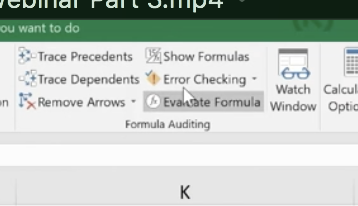
Or to find any errors, go to Formula Auditing in the top menu.
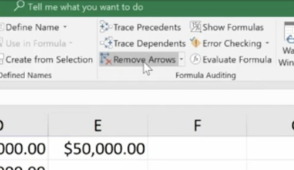
You have a number of helpful tools here. Trace Precedents shows where the formula looks for information. Click the formula you want and click Trace Precedents. It will display where your data came from.
Here’s a more complex formula and trace auditing:
To hide the arrows, click “Remove Arrows.”
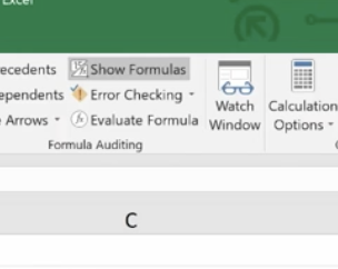
Show Formulas
This expands all of your columns and shows all of them in a bigger way. You can go in and check your formulas on the fly very easily. Click Show Formulas again and the worksheet goes back to the way it was before.
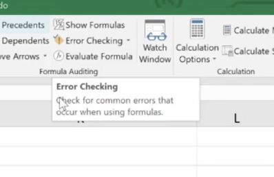
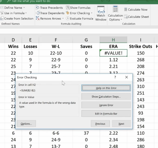
Error Checking
This feature lets you check all formulas at once.
This makes it easy to find errors and correct them.
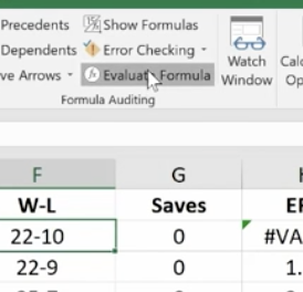
Evaluate Formula
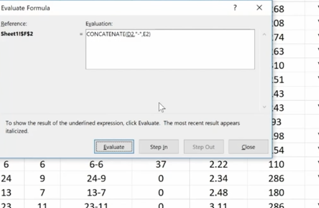
This feature allows you to check a formula step-by-step. It shows the results of each individual part. It’s another great way to de-bug a formula that isn’t working for you. Click the formula you want to evaluate. Click Evaluate Formula and you’ll get a dialog box.
Click Evaluate and it will change the formula to the actual value that you can review. Each time you click Evaluate, it will take you through the steps of how you got to the final formula. You can trace your way through to see if you made any errors.
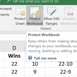
Protection
With protection you can lock in your changes in individual cells, spreadsheets, and entire workbooks. You can also protect comments from being moved or edited.
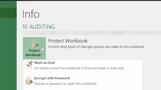
This is how to protect an entire workbook. It’s the highest level of protection.
You’ll want to do this if your workbook contains confidential information like:
Pre-released quarterly results
Employee salary tables
Staff member evaluations
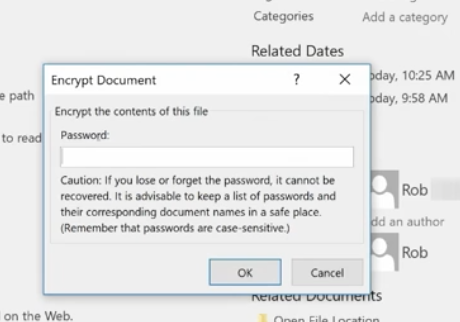
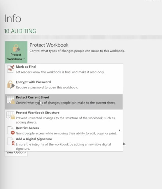
Click File>Info>Protect Workbook>Encrypt with Password.
Enter your password and be sure to make note of it because it can’t be recovered if you lose it. You can use password management software to keep track of your passwords.
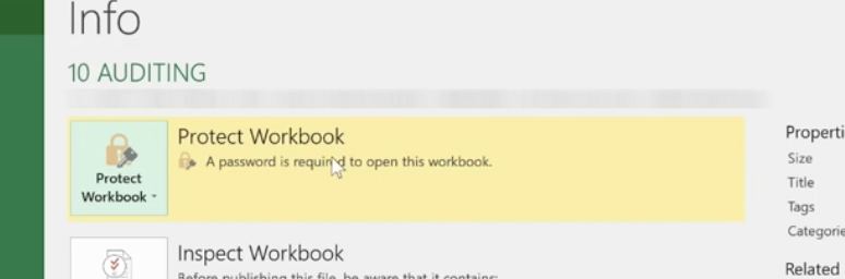
Once complete, click OK and your Protect Workbook function turns yellow indicating that you’ve protected your workbook.
To take off protection, retrace your steps.
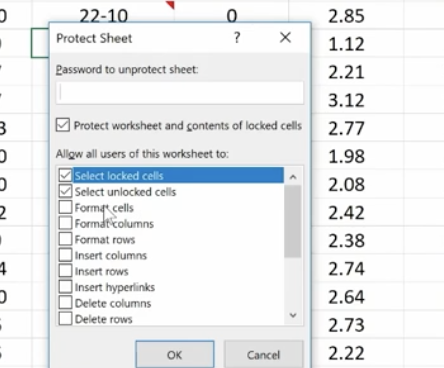
You can also protect a current sheet you’re working on. It will take you back to your worksheet where you’ll be presented with a variety of options.
You can also protect cells and comments from this option.
In the same way you protected the worksheet, you can protect your workbook.
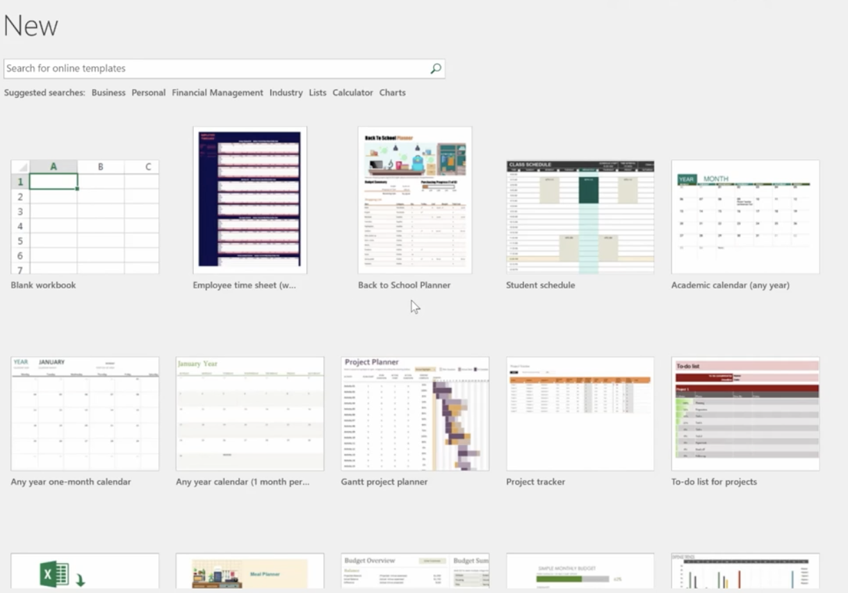
Using Templates
To see the variety of templates you can use in Excel, click File>New and you’ll be presented with a collection of 25 templates you can choose from.
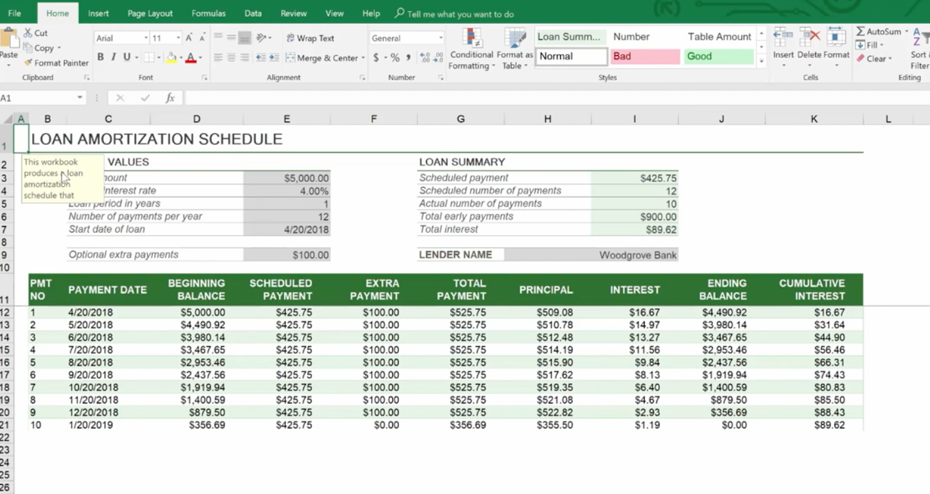
For example, there’s a great Loan Amortization Schedule you can use. Formulas are built in for you. All you need to do is change the numbers.
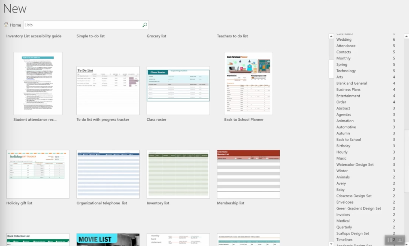
You can also go online while inside Excel to find more. You don’t want to download templates from outside Excel because they may contain macros that are contaminated with viruses.
On the right side of the page, you have a huge selection to choose from.
It even provides employee time sheets you can use that can save you so much time trying to figure out formulas.
Creating and Managing Templates
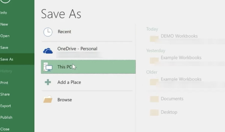
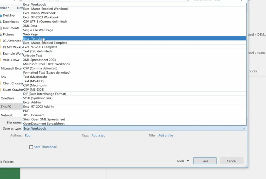
Go to File>Info>Save As and save the template to your location, then save as an Excel Template.
Before you save as a template you want to:
Finalize the look and feel of your template
Use review and auditing tools
Remove unnecessary data and information
Unprotect cells and sheets as appropriate
Create comments as guides
Congratulations! Now you’re an Excel Pro! This completes our Excel Like a Pro Series. If you have any questions or need assistance, feel free to contact our Excel 2016 experts.
Microsoft introduced the Surface Pro 4 Tablet some time back in 2015. It replaced an older model called the Surface Pro. Soon after the release of the Surface Pro 4, Microsoft’s social media pages were flooded with complaints about a flickering screen. The Redmond Washington-based company responded to these complaints by promising that they would replace some Surface Pro 4 devices with this problem.
Trouble for the tech giant
This is good news especially since the company is making the replacements for free, but for only those devices experiencing the mishap within three years of purchase. In their web page called Surface Pro 4 screen flickers [https://support.microsoft.com/en-us/help/4230448/surface-pro-4-screen-flicker], Microsoft said that their top priority is to create the best products and experiences for their customers. Further, the company noted that they have heard their customer’s complaints and that’s why they have come on board to address these issues. After some investigation, Microsoft determined that some of the affected Surface Pro 4 devices could not be repaired with driver updates or new firmware.
Surface Pro 4 users who are experiencing the flicker are advised to first install the latest Surface and Windows programs to ensure that this is not the cause of the flickering. Surface and Windows updates are designed to keep any device running in an optimal state. If the issue persists, consumers should contact Microsoft Support. Once they verify that the device is certified as one of those that will require a replacement, the exchange process is set in motion.
Getting your Surface Pro 4 replaced or repaired
For those shipping their devices out to Microsoft for repair or replacement, it typically takes about 5-8 business days for the tech giant to get your broken device. The time to repair or replace it can vary depending upon several different factors. Microsoft has also promised to refund the warranty fee to customers who paid for a warranty fee to repair their device. In order to get a refund, customers must contact Customer Support for validation. Microsoft is committed to delivering great products and services to their customers.
Consumer complaints
Information about the flickering screen issue came to the attention of Microsoft after Consumer Reports, a non-profit organization that offers product ratings, said that they could no longer recommend Microsoft Surface products because the device did not perform as expected. As any serious service provider would do, Microsoft did a thorough examination, made their own findings, and came up with a resolution to have the screen replacement performed for free.
Further, Consumer Reports learned about the flickering screen from surveyed electronic owners who said that their Surface Pro had too many problems and that they would not recommend it. Experts have been concerned that the Surface Book Laptop may be more likely to have screen failures as compared to other competing brands. To date, this has not been the case, but it has caused sales of these products to decline.
Mitigating the damages
Microsoft’s decision to replace the flickering screens for free might not be the immediate solution that will stop future damage, but they are hoping to mitigate the harm caused by negative reviews of the Surface Pro devices. Nothing raises the spirits of a devoted customer or consumer than a company that acknowledges fault on their part and gives a remedy with no strings attached.
Many companies, especially those in the business of electronic devices, handle these types of issues poorly. They often spend months denying that anything is wrong. Then, later they make the method of repair and replacement so complicated that users get frustrated. Some warranties are felt to be useless due to these and other problems that people have experienced over the years. Consumers often complain that no one seems to qualify for the free repair services.
However, with the Microsoft Surface Pro 4, the steps were purposely made simple and straightforward. This encouraged those affected to give the company a second chance to do it right. Often, this type of issue can turn off consumers to a product or even an entire brand, but Microsoft has made every attempt to do the right thing.
Future Microsoft designs
The Microsoft design team has taken these problems into consideration when developing new versions of the Surface Pro. For the future, Microsoft products should have very clear and reliable screens that will last for years with no problems. The company seems to have learned an important lesson throughout this ordeal.
Developing brand loyalty
What Microsoft has done by launching the Surface Pro 4 Replacement Program is not only a wise corporate decision, but a show of gratitude and humility to their consumers. This is probably a major reason why Microsoft customers are loyal to this brand. They expect perfection from the company and do not accept anything less.
With everyone so busy these days, people are searching for new ways to get more done and Microsoft Planner is an excellent tool for that. It allows teams and individuals to collaborate on any project in real time. It has so many great features that can streamline projects, helping you to achieve deadlines while producing better work.
Each year, Microsoft works diligently to update its product line with helpful features for all products including its Planner. These features are designed to give users greater insight into project schedules, receive notifications of upcoming deadlines, and filter tasks accordingly.
The latest and one of the most useful features for the Microsoft Planner enables users to publish tasks to their Outlook calendar. This handy feature allows users to view their Outlook calendar alongside their personal calendar. This can give you a much better idea of what’s coming up and what projects you need to work on first.
There are numerous other features like this that can cut time and stress out of your day. Since many are not familiar with these new functions, we’re going over them to give users a bird’s eye view of some of the most important new updates in MS Planner.
First things first: what to know about Microsoft Planner
MS Planner is a sophisticated work management app that comes as part of Office 365. Today, millions of businesses and offices worldwide are using Office 365. This product is part of Microsoft’s cloud-based environment that includes well-known programs such as Word, PowerPoint, Excel and OneNote.
MS Planner offers its users the ability to organize any project, share files with others or even collaborate on a project. It features a very handy chat environment where employees can get together and discuss a project while jointly viewing files.
The Outlook Calendar
As a busy individual, you are probably looking for anything that can make your life simpler. Having a work calendar that integrates with your personal calendar is a big time-saver. You can now view or import Planner tasks into your Outlook calendar. Adding the task to your Outlook calendar can be accomplished using the iCalendar feed. This creates a link that members can share with others.
Publishing an iCalendar feed is simple as well. Start by tapping the ellipsis at the top of your page, then select the Add plan to Outlook calendar from the drop-down menu. A dialog box appears giving you the option to Publish or Unpublish your plan’s schedule and other information. By selecting Publish, you can automatically send scheduling information to anyone with the iCalendar link. Now that person can open the plan in their own personal Outlook program.
Please note that you must be the plan owner in order to view and work with this feature. In addition, your admin has the ability to turn this feature off when setting up MS Planner.
Visually organizing your work
MS Planner allows users to organize their tasks into buckets. This feature makes it easy to categorize each task based on several factors. A task can be organized by the task owner, the status, the due date and other dynamics. You can designate a task as a Favorite or check to see which tasks are due first. Updating the status of any assignment or handing it off to another staff member is easy to do because tasks in Planner can be dragged and dropped between columns.
You might want to check and see who’s working on a specific task or whether a task is overdue. Each plan has its own Board with Charts view. By checking the Charts view, users can see the overall progress of the task. Who’s been working on it? What still needs to be done? The Charts view gives you lots of important information about any task.
Adding iCalendar link to Outlook
Click on the option called Add to Outlook to add the plan to your own Outlook calendar. This prompt opens up your personal Outlook calendar in Outlook on the web. The dialog box contains the same iCalendar link and the calendar name (which you can change if you’d like to rename the plan.) Once you’ve created an iCalendar link, you can then paste it into any iCalendar app. Users who have the link can easily view your plan’s task information.
Adding a plan to your Outlook calendar if not the plan owner
Sometimes the plan owner will want to share their iCalendar link with you so that you can add it to your personal Outlook calendar. To accomplish this, click on the ellipsis at the top of the plan and select Add plan to Outlook calendar in the drop-down menu that appears. Now you’ll have the option to review everything before saving it. Once the plan is saved, all info is imported to Outlook. You can view the details using Outlook. The plan now appears under People’s calendars. Select the plan to view all the details.
At nearly $1 Trillion in earnings a year, hacking is now at record proportions. Your data is a valuable asset, not only to you but to criminals as well. Don’t get hacked.
Here’s what you need to know.
1 in 3 Americans has been hacked.
A hacker attacks someone every 39 seconds.
61% of small businesses experienced a cyber-attack within the past year.
The average cost of a data breach in the U.S. is $7.35 Million.
$5 Billion was lost due to hacking in 2017. This is more than 15 times the total losses in 2016. Most of this cost was due to data breach fines, downtime, and productivity losses.
54% of breaches are caused by negligent employees who click on suspicious websites and emails.
20% of businesses experienced downtime of over 100 hours due to ransomware attacks.
64% of businesses paid ransoms even though paying doesn’t guarantee that data will be returned.
The anticipated cost of cybercrime in the next 3 years is$6 Trillion.
The pool of cybersecurity experts is shrinking. By 2021 there will be 3.5 Millionjobs that can’t be filled. The demand for security experts is increasing and is outpacing the supply.
5 THINGS TO DO RIGHT NOW
Ignore Ransomware Threat Popups and Don’t Fall for Phishing Attacks.
These attacks say that your data will be encrypted so you can’t access it, but in many cases, this isn’t true; it’s just a ploy to get you to click on something harmful. Once you click on the link, then you’re in trouble. You may have to pay a ransom to get your files unlocked.
Ransomware is a type of malicious software (malware) that blocks access to a computer. It infects, locks, or takes control of a system and demands a ransom to unlock it. It’s also referred to as a crypto-virus, crypto-Trojan or crypto-worm. It then threatens that your data will be gone forever if you don’t pay using a form of anonymous online currency such as Bitcoin.
Phishing is when a scammer uses fraudulent emails, texts, or copycat websites to get you to click a link so they can steal your confidential information. Thieves are looking for information like social security numbers, account numbers, login IDs, and passwords. They use this information to rob you of your money and your identity. The odds are good that phishing will work. A campaign of 10 messages has a better than 90% chance of getting clicked on. The majority of account takeovers come from simple phishing attacks where you or someone in your organization gets tricked into releasing private credentials and information.
Use Hard-to-Guess Passwords and Two-Factor Authentication.
Use complex passwords with 9+ characters and don’t reuse passwords across your different accounts. Consider using a password manager like LastPass. For accounts that support this, two-factor authentication is an extra step worth taking to ensure the privacy of your data. It requires both your password and an additional piece of information to log in to an account. The second piece could be a code the company sends to your phone or a random number generated by an application or token. Two-factor authentication will protect your account even if your password is compromised.
Secure Wi-Fi With a Virtual Private Network (VPN).
Hackers now emulate free open Wi-Fi to steal your IDs and passwords. You can be fooled when you try to login to free Wi-Fi in airports, restaurants, and other public areas. When this happens, everything that you type is copied and archived by these criminals and used against you. Using a VPN encrypts your Internet connection and protects your privacy. When you connect to the Wi-Fi over your Virtual Private Network, no one can see the information you send, and your privacy is safeguarded at all times.
Back Up Your Data.
Store data both onsite and offsite in a secure Enterprise-Based Cloud System. Back up your files regularly to ensure you have a duplicate of all your files and applications if your network is compromised. Traditional data backups can’t always restore all of an IT system’s data and settings. This is why you need both an onsite backup and a reliable backup via the Cloud. An enterprise-based cloud backup solution safeguards your data and ensures that it’s recoverable under any circumstance.
Hire a Reputable Technology Solutions Provider to Help.
A reputable Technology Solutions Provider can deploy a layered security protocol with regular software patches, vulnerability management, and continuously-updated endpoint protection. They can also provide Security Awareness Training for your employees to help them recognize potential threats. With the right provider, you’ll boost your defense posture and decrease the likelihood that a data breach will take down your business.
Don’t get hacked. Contact us, and we’ll keep your data secure.
This is the final of a three-part series about using Microsoft Excel 2016. It will cover some of the more advanced topics. If you aren’t great with numbers, don’t worry. Excel does the work for you. With the 2016 version of Excel, Microsoft really upped its game. Excel’s easy one-click access can be customized to provide the functionality you need.
If you haven’t read Part I and Part II of this series, it’s suggested that you do so. The webinar versions can also be found on our site or on YouTube.
This session will discuss the following:
More with Functions and Formulas
Naming Cells and Cell Ranges
Statistical Functions
Lookup and Reference Functions
Text Functions
Documenting and Auditing
Commenting
Auditing Features
Protection
Using Templates
Built-In Templates
Creating and Managing Templates
More With Functions And Formulas
Naming Cells And Cell Ranges
How do you name a cell? You do so by the cell’s coordinates, such as A2 or B3, etc. When you write formulas using Excel’s coordinates and ranges you are “speaking” Excel’s language. However, this can be cumbersome. For example, here G12 is significant because it refers to our Team Sales.
You can teach Excel to speak your language by naming the G12 cell Team Sales. This will have more meaning to you and your teammates. The benefits of naming cells in this fashion are that they are easier to remember, reduce the likelihood of errors, and use absolute references (by default).
To name our G12 cell Team Sales, right-click on the cell, choose Define Name, and type “Team Sales” into the dialog box. You can also add any comments you want here. Then click Ok.
Another way to do this is to click on the G12 cell and go up to the Name Box next to the Formula Bar, then type your name there.
And, there’s a third option at the top of the page called “Define Cells” that you can use.
Notice that there’s an underscore between Team and Sales (Team_Sales). There are some rules around naming cells:
You’re capped at 255 characters.
The names must start with a letter, underscore or a backslash (\).
You can only use letters, numbers, underscores or periods.
Strings that are the same as a cell reference, for example B1, or have any of the following single letters (C,c,R,r) cannot be used as names.
How To Name A Range
Highlight an entire range of cells and name your range (we’re doing this in the upper left-hand corner).
Then you can easily use the name to produce the sum you need:
You won’t have to go back and forth from spreadsheet to spreadsheet clicking on specific cells to calculate your formula. You simply key in the name of the cell range you want to add. Just be sure to remember the names as you build your spreadsheets over time.
If you ever make a mistake or want to change names, you can go to Name Manager to do this.
Remember that if you move the cells, the name goes with it.
Statistical Functions
The three statistical functions are:
Average If
Count If
Sum If
The Average If can be used to figure out the average of a range based on certain criteria. Here we’re going calculate the Average If of the ERA of 20+ Game Winners from the spreadsheet we developed in our last session.
We’ve already named some of our cell ranges (wins, era). And we want to know the average greater than 19.
Hit Enter and you have the average.
You can use this feature across a wide variety of scenarios. For example, if you wanted to know the average sales of orders above a certain quantity – or units sold by a particular region, or the average profit by a distinct quarter.
Count If is used for finding answers to questions like, “How many orders did client x place?” “How many sales reps had sales of $1,000 or more this week?” or “How many times have the pitchers of the Philadelphia Phillies won the Cy Young Award?”
As you can imagine, it’s essential that you type in the text exactly the way you named that particular cell.
Hit Enter and you get your answer
Now we’re going to use the Sum If function to calculate the number of strikeouts by the pitchers on this list who are in the Baseball Hall of Fame.
Sum If is a good way to perform a number of real-world statistical analyses. For example, total commissions on sales above a certain price, or total bonuses due to reps who met a target goal, or total earnings in a particular quarter year-over-year.
Lookup and Reference Functions
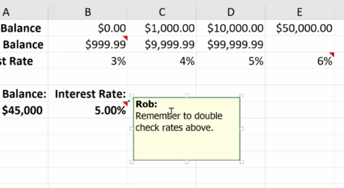
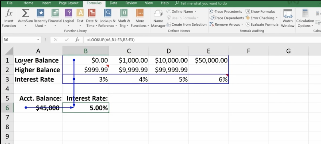
These are designed to ease the finding and referencing of data, especially in large tables. Here, cells A1 and E3 relate to a variable interest rate that is paid on a bank account. For balances under $1,000, the interest rate is 3% – between $1,000 and $10,000, the interest rate is 4%, etc.
Cell A6 shows the balance of a specific account. The Lookup Function is used in B6. It looks up the interest rate and applies it to the account balance of $45,000. This is what the formula looks like in the bar at the top:
The vector form of the Excel Lookup Function can be used with any two arrays of data that have one-to-one matching values. For example, two columns of data, two rows of data, or even a column and a row would work, as long as the Lookup Vector is ordered (alphabetically or numerically), and the two data sets are the same length.
V Lookup and H Lookup are used to pull information into reports. We’re going to use Report Setup. Here, we have a worksheet that references salespeople, sales data, pricing, revenue, and the clients that they sold to. You’ll see on the top right where we set up a report with names referencing sales data.
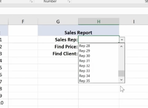
You can access the sales reps in the drop-down menu. Pick a rep and use the V Lookup Function to find the price.
To Find Price, key in =vlookup and the corresponding cell number for Rep 16, plus the table array which is the entire table not including the header at the top.
Then you need the column index number. This is the number of columns to the right of your lookup value column, which is column A. It’s the 4th column from column A (Price).
Enter 4,
For range lookup we’re using true or false. We are entering false here.
Hit Enter and this is what you have for your Find Price value.
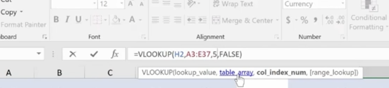
Now we’ll do a similar V Lookup for the Client. Copy and Paste:
Make the necessary changes in your formula:
Client 16 goes with Rep 16.
Note: If you change the Sales Rep, all the corresponding values will change.
If you have a lot of data and long tables, V Lookup helps you find information easily. The V stands for Vertical (or by column), because columns are vertical. H Lookup is for Horizontal-like column headers.
Text Functions
Text Functions contain some very powerful tools to adjust, rearrange and even combine data. These functions are used for worksheets that contain information and function as a database such as mailing lists, product catalogs, or even Cy Young Award Winners.
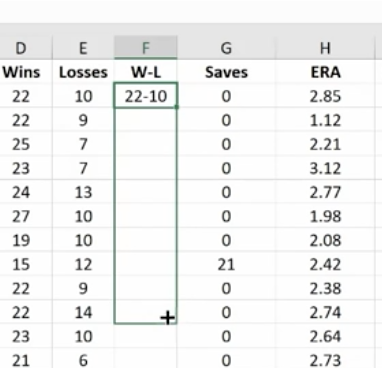
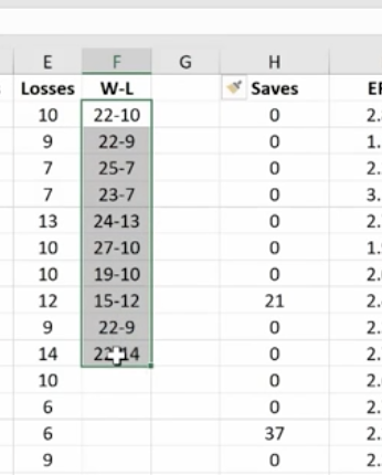
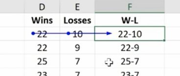
The first text function we’ll show you is concatenate. It links things together in a chain or series. Here, we have our Cy Young list. But we no longer need to see our Wins and Losses in a separate column.
To do this easily rather than manually, create a new column where your data will reside.
Hit Enter
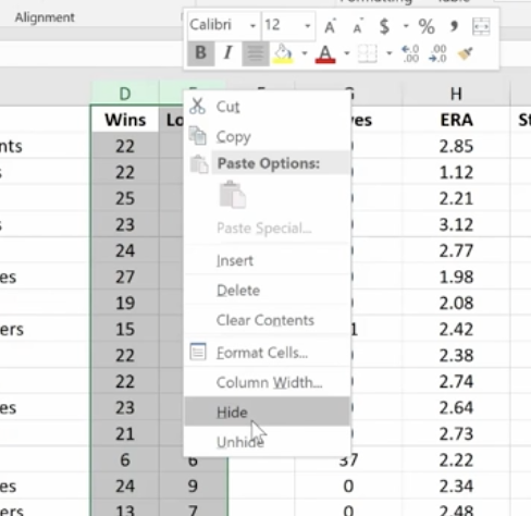
Now, just go in and hide the Wins and Losses columns. Don’t delete them or your new column will have a reference error.
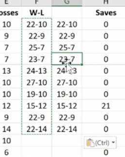
If you do want to delete the Wins and Losses columns, you must first make a new column. Copy the W-L numbers and Paste Value in the new column. This way you’ve moved from a formula to the new information. If you delete your source information without taking this step you’ll be left with nothing.
Combine as many columns as you need with the concatenate function to make the data appear as you need it to.
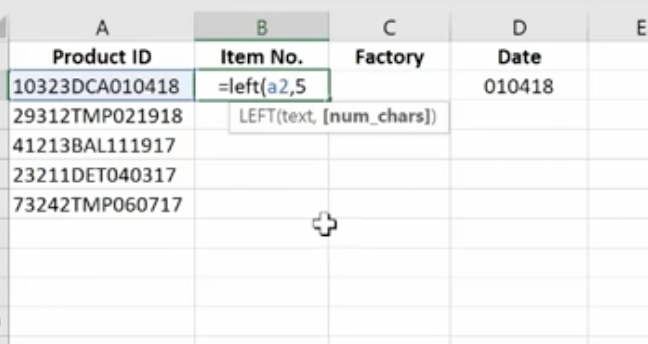
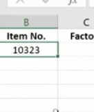
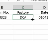
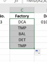
The Left Mid and Right Functions
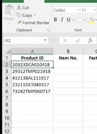
These are used to tell Excel that you only want part of a text string in a particular cell. Here, we have a product list and product IDs that tell us the date of manufacturer, the item number, and the factory where it was made. We’re going to pull the data out so we can put it in columns to use in different ways.
We use the Mid Function here.
This works because each of the product IDs are the same length. If they were different lengths you’d have to do something more creative.
Documenting and Auditing
You want to make your Excel files easy to understand for both yourself and others who need to use them – and this includes auditors. An organized worksheet results in clear error-free data and functions.
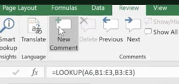
Commenting
The purpose of commenting is to provide notes to yourself or especially to others. Comments can include reminders, explanations or suggestions.
You’ll find the New Comment button at the top under the Review Menu. Simply click the cell where you want the comment to go and click New Comment. Then type your comment and click outside the box to close it. The comment will disappear but it’s still there. Anywhere you see a red flag, there’s a comment.
If your name doesn’t appear in the comment, go to File>Options>General and personalize your copy of Excel (in this case Microsoft Office) under the User Name. You won’t need to go back and change each comment; Excel will do this for you.
To format a comment, click inside the comment box and a drop down will come up where you can format the text.
You can change the color of the box and lines around the box. Some managers have different colors for members of their teams.
If you change the default color, it will change that for all your Microsoft products.
To delete a comment, go to the cell that hosts it, then go up and hit delete.
If you have a lot of comments, grab the handle on the box and resize it.
Auditing
What we really mean is formula auditing. This is an advanced way to check your work.
The yellow diamond on the left of this cell indicates that there’s an error.
Or to find any errors, go to Formula Auditing in the top menu.
You have a number of helpful tools here. Trace Precedents shows where the formula looks for information. Click the formula you want and click Trace Precedents. It will display where your data came from.
Here’s a more complex formula and trace auditing:
To hide the arrows, click “Remove Arrows.”
Show Formulas
This expands all of your columns and shows all of them in a bigger way. You can go in and check your formulas on the fly very easily. Click Show Formulas again and the worksheet goes back to the way it was before.
Error Checking
This feature lets you check all formulas at once.
This makes it easy to find errors and correct them.
Evaluate Formula
This feature allows you to check a formula step-by-step. It shows the results of each individual part. It’s another great way to de-bug a formula that isn’t working for you. Click the formula you want to evaluate. Click Evaluate Formula and you’ll get a dialog box.
Click Evaluate and it will change the formula to the actual value that you can review. Each time you click Evaluate, it will take you through the steps of how you got to the final formula. You can trace your way through to see if you made any errors.
Protection
With protection you can lock in your changes in individual cells, spreadsheets, and entire workbooks. You can also protect comments from being moved or edited.
This is how to protect an entire workbook. It’s the highest level of protection.
You’ll want to do this if your workbook contains confidential information like:
Pre-released quarterly results
Employee salary tables
Staff member evaluations
Click File>Info>Protect Workbook>Encrypt with Password.
Enter your password and be sure to make note of it because it can’t be recovered if you lose it. You can use password management software to keep track of your passwords.
Once complete, click OK and your Protect Workbook function turns yellow indicating that you’ve protected your workbook.
To take off protection, retrace your steps.
You can also protect a current sheet you’re working on. It will take you back to your worksheet where you’ll be presented with a variety of options.
You can also protect cells and comments from this option.
In the same way you protected the worksheet, you can protect your workbook.
Using Templates
To see the variety of templates you can use in Excel, click File>New and you’ll be presented with a collection of 25 templates you can choose from.
For example, there’s a great Loan Amortization Schedule you can use. Formulas are built in for you. All you need to do is change the numbers.
You can also go online while inside Excel to find more. You don’t want to download templates from outside Excel because they may contain macros that are contaminated with viruses.
On the right side of the page, you have a huge selection to choose from.
It even provides employee time sheets you can use that can save you so much time trying to figure out formulas.
Creating and Managing Templates
Go to File>Info>Save As and save the template to your location, then save as an Excel Template.
Before you save as a template you want to:
Finalize the look and feel of your template
Use review and auditing tools
Remove unnecessary data and information
Unprotect cells and sheets as appropriate
Create comments as guides
Congratulations! Now you’re an Excel Pro! This completes our Excel Like a Pro Series. If you have any questions or need assistance, feel free to contact our Excel 2016 experts.


 Phishing is one of the most dangerous forms of identity theft. It’s usually presented in the form of pop-ups or spam emails. The majority of account takeovers come from simple phishing attacks where someone in an organization gets tricked into releasing private credentials and information.